Homework no. 4

Here’s the Python-Screenshot.

And below is a short proposal I recently wrote. You can download the pdf here and the odt here.

Introduction

We tend to think about the category of “the sciences” as divided into thematic units. Chemists deal with molecules, economists with money, biologists with living things, physicists with matter and psychologists with the human experience and behaviour. These units can be divided into sub-units, like particle-physics, organic chemistry or developmental psychology. And they can, on rare occasions be matched more or less fruitfully, as it is the case with behavioural economics, evolutionary psychology, astrobiology etc.¹ But it is not clear, whether this top-down-classification, which seems to be rooted in deep metaphysical assumptions² matches the structure of the knowledge which is actually produced by scientists.

Humphreys (2002) suggests that a better tool for the taxonomisation of the sciences might actually be their usage of computational templates (Humphreys 2002, 5). This paper will describe and conduct a computational approach to find out whether such a taxonomization would be feasible, and whether we could expect for it to align itself well with the ‘standard-picture’ of the sciences.

The Data

In order to test this hypothesis, I have downloaded the most recent 76900 papers from the preprint server ArXive via data dumps that were uploaded to the Internet-Archive (“arXiv.Org Bulk Content : Free Texts : Free Download, Borrow and Streaming : Internet Archive,” n.d.).³ All papers were in the format of \LaTeX documents. Historically ArXive archives mainly papers from physics, but recently there has been a significant influx of papers form economics, computational biology, linguistics, computer- and cognitive-science. This provides a good opportunity for us, as most disciplines where we can expect to find usage of formulas or computational templates will probably be present – although not as exhaustively as physics.

Processing the Formulaic Structure

In the original abstract the use of distance measures between formulas was proposed. The trouble with these attempts was, that they had a way to high time-complexity, at least $O(n^2)$, in some cases $O(n^4)$, which is why a Bag-of-Words-paradigm was used instead.

To avoid the computation of each individual link, a vocabulary of equation-particles (the ‘words’) was constructed. For a set number of instances (a few hundred thousand), two random papers where selected, their formulaic content extracted, and the largest common substring of those formulas was saved off. These largest common substrings where in many cases simple building-blocks of equations, like \rightarrow which translates to the \LaTeX symbol ‘$\rightarrow$’, or \frac{1}{2}, which represents ‘$\frac{1}{2}$’. These contain of course little interesting information, and can be considered similar to the so called stopwords in natural language programming – words like ‘and’, ‘or’, ‘the’, etc. – which add little to our understanding of the content of a text. More interesting are the slightly rarer occurences of particles like $\frac{1}{\sqrt{2}}$ or $(2\pi)^3$. But here are even larger shared equations, like, e.g. $({Q^2+a})^{1+\Delta(Q^2)}$ or, already quite rare, $\frac{\sigma_{ab}}{\sigma_{c}}=\frac{\ell^2}{\ell_c^2}. \frac{\sigma_{ab}}{\bar\sigma }=f\left (\frac{\ell}{\bar\ell}\right)$. A great advantage of this approach is, that it can, to a certain extent, ignore variable names – some authors might e.g choose to explicate the same model with Greek instead of roman letters, or use $i$ as a counting variable, where others might use $n$ – , as the particles that are grouped around the variables are kept for analysis.

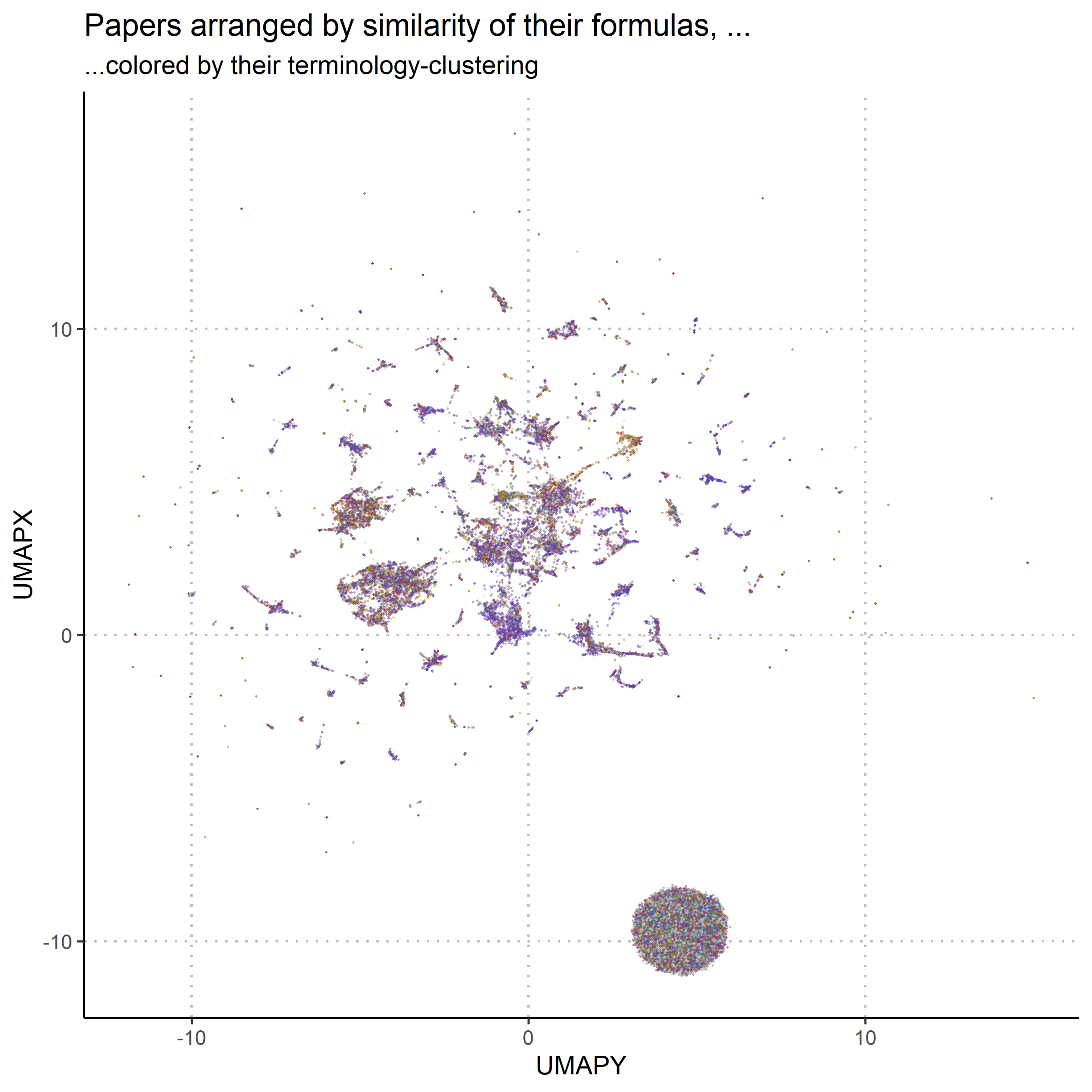
An inexpensive way to get rid of the formulas “stopwords”, the particles that are so common that they contain barely any information, is to conduct Principal Component Analysis on the document vectors, and then to remove the five components that explain the most of the variance, a “trick” described by Arora, Liang, and Ma (2017). The so altered data then underwent non-linear dimensionality-reduction with UMAP (McInnes, Healy, and Melville 2018). UMAP constructs a weighted k-neighbour graph, which means that for each article, it looks up the $k=50$ nearest other articles according to a similarity measure, in our case cosine similarity and converts this measure to a connection between the two of a certain strength. If in the formulas of a paper occurs for example the particle $g^{\mu\nu}$, it will have a rather strong connection to all the papers in which the same particle occurs. The next step to give a representation of that graph in a low-dimensional space, which can be directly perceived by us as a two dimensional mapping. For this, UMAP uses a force-directed layout: All articles are assigned coordinates, and then moved around like balls connected with springs, which push and pull them until an optimal state is reached, in which strongly linked papers are in close proximity. The result of this process is shown in figure 1. Each point represents a paper, positioned according to its relation to the surrounding papers (It should be noted that the x- and y-values are completely meaningless in UMAP-plots. Only the relations between the points count.). It is pretty clear that the algorithm has found a lot structure in the dataset. The black ball in the lower right corner consists of all the documents which contained no formulas, grouped close together, because they are of course very similar. The rest of the documents, on the other hand, clearly form an interesting structure, which is not uniform but divided into interconnected groups. This can considered strong evidence that a taxonomy of scientific literature through the use of computational templates is indeed possible. Now it will be investigated how it relates to the thematic structure of the literature.

The Thematic Structure

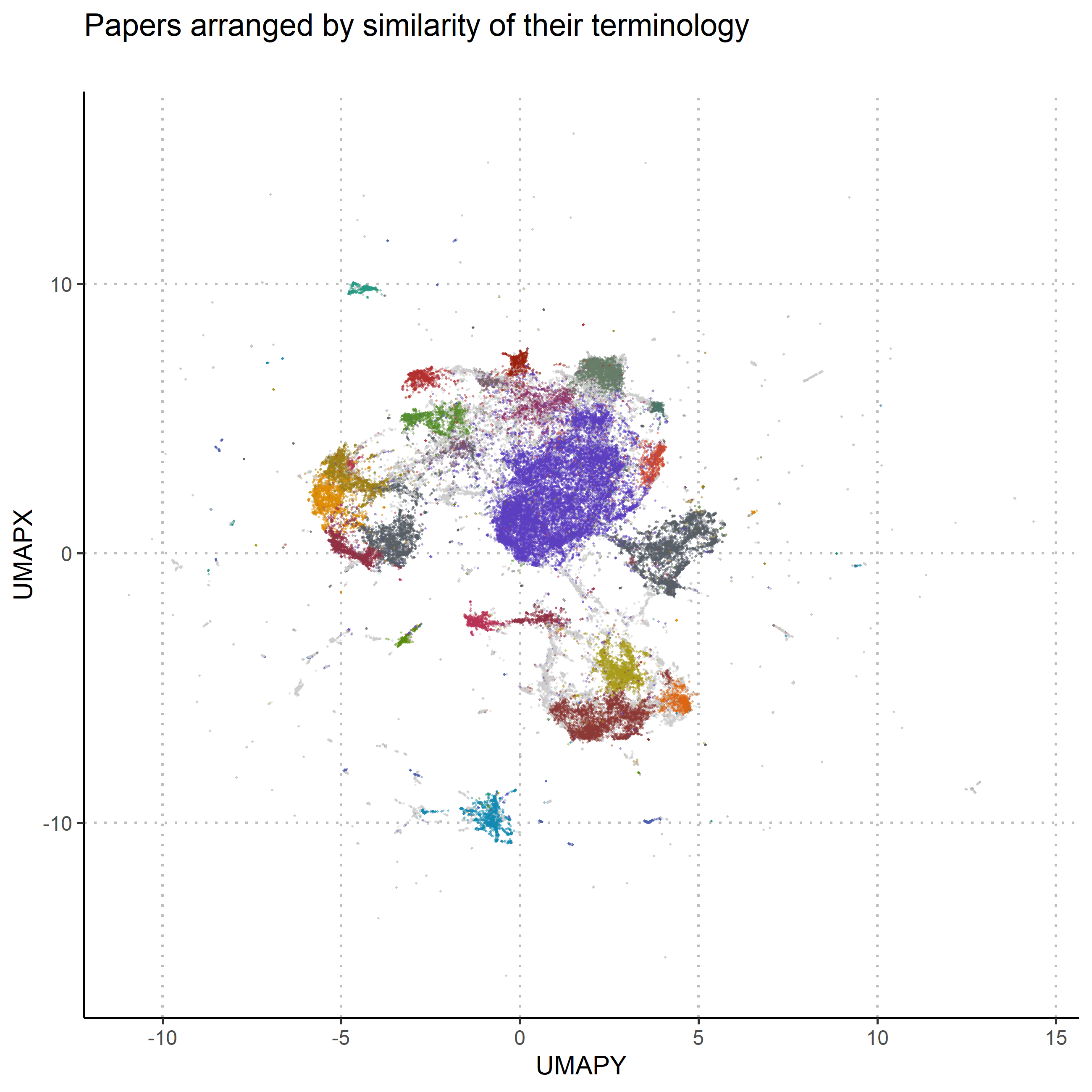
To compare the thematic structure to the formulaic one, the exactly same process was employed, with the only difference being that instead of formula-particles, the actual words in the papers⁴ were used, and that the results were not only layed out with umap, but also clustered with hDBSCAN (McInnes, Healy, and Astels 2017). The results are displayed in figure two. Again each datapoint represents a paper, coloured according to the cluster the algorithm assigned it to. Grey datapoints were considered noise by the algorithm. Datapoints close to each other represent papers that use the same words. Noticeably the round ball from the formulaic structure is missing as, unsurprisingly, there were no papers without text. Also the overall texture is smoother, presumably because the data is much more densely interrelated.

Results

To finally see how the formulaic structure and the thematic structure hold up against each other, the thematic clustering is projected onto the formulaic structure: The papers in figure 1 are coloured with the colour they received in figure 2. The match is, as can be seen in figure 3, not good. On close inspection it is possible to discern areas where there might be some prevalence over one colour over the others, but in total, the two structures don’t really match up. This suggests that the taxonomy, which Humphrey is proposing would indeed be very different from the standard picture. To summarise these findings:

1. The mathematized sciences are structured by the computational templates they use. Computational templates are not distributed uniformly through science.
2. This structure does not match the thematic structure of science, as expressed through the words in scientific articles.

Further work

There are several things which could not be satisfactorily addressed in this short paper. The most prominent concern is of course the question on how to get back from the splitters of formulas back to equations or models, or in other words, how to learn more about this separate structure of science. It should also be investigated, what the clusters displayed in figure 2 actually contain. And while the graphical illustration brings a certain satisfaction with it, to make a strong argument about how the two structures match up, it would be necessary to come up with an actual tatistical index of how well they match up.⁵

To gain more confidence in the presented results, it would also be necessary to give a good account of the actual content of our dataset in terms of its meta-data: How exactly is its temporal distribution? What discipline were the papers actually assigned to, and where have they been ultimately published? What happens when we account for different \LaTeX-styles? And finally: What would we learn if we were to work on the whole dataset of more than a million preprints? At the moment I don’t possess the resources to answer this. Downloading and preprocessing of that data alone should take with my connection around twenty days.

Literature

Arora, Sanjeev, Yingyu Liang, and Tengyu Ma. 2017. “A Simple but Tough-to-Beat Baseline for Sentence Embeddings,” 16.

“arXiv.Org Bulk Content : Free Texts : Free Download, Borrow and Streaming : Internet Archive.” n.d. https://archive.org/details/arxiv-bulk?sort=-publicdate.

“Branches of Science.” 2019. Wikipedia, August.

Humphreys, Paul. 2002. “Computational Models.” Philosophy of Science 69 (S3): S1–S11. https://doi.org/10.1086/341763.

McInnes, Leland, John Healy, and Steve Astels. 2017. “Hdbscan: Hierarchical Density Based Clustering.” The Journal of Open Source Software 2 (11): 205. https://doi.org/10.21105/joss.00205.

McInnes, Leland, John Healy, and James Melville. 2018. “UMAP: Uniform Manifold Approximation and Projection for Dimension Reduction.” arXiv:1802.03426 [Cs, Stat], February. http://arxiv.org/abs/1802.03426.

Rand, William M. 1971. “Objective Criteria for the Evaluation of Clustering Methods.” Journal of the American Statistical Association 66 (336): 846–50. https://doi.org/10.1080/01621459.1971.10482356.

---